The Canvas and its optional views
Most nodes and inputs use a canvas to display some bands of an image as RGB. This will take up a large proportion of their view - in some cases all of it. It is worth discussing in some detail. A canvas is shown below as the entire control area for an input node, which brings one of the four inputs into the graph.
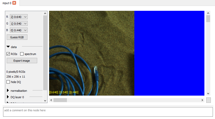
You can pan the canvas using the scroll bars at the edge, by holding down the middle mouse button and dragging, or with the keyboard (see below). You can zoom with the mouse wheel or the keyboard.
Canvas corner buttons
The "two arrows" button at bottom right will reset to show the entire image.
The S button will save the coordinates of the current view, while the L button will load saved coordinates into the current view. This can be very useful when you are looking at a small part of an image, and wish to look at the same part of the image in another node.
Keyboard control
If the canvas has focus (click on it first), you can also pan and zoom using the keyboard - handy if you're on a laptop without a scroll wheel or middle mouse button:
- Arrow keys pan the view. Hold Shift for a finer pan, or Ctrl for a coarser one.
- +/= and - zoom in and out.
- 0 resets the zoom and pan to show the entire image (the same as the reset button).
Some nodes use the arrow keys for their own purposes when their tab is showing the canvas -
for example, stitch uses plain/Shift/Ctrl + arrow keys to fine-tune the position of the
selected input image - so keyboard panning isn't available on those particular tabs. Zoom
keys (+/-/0) are unaffected and still work everywhere.
To the left of the canvas image itself is the canvas control area. This has quite a lot in it, so is scrollable with collapsible sections, rather like the palette.
At the top - and not collapsible - are three combo boxes which determine the image mapping : how the bands within the (probably) multispectral image map onto RGB channels for viewing. Each band in the combo box shows the input number (i.e. which of the four global inputs the data is sourced from), a colon, and typically the name, position or wavelength of the band. Exactly what is shown depends on the image being loaded and the Caption global control. The Guess RGB button tries to guess appropriate channels for the RGB canvas image.
Data section
This is the first of the collapsible sections.
- Show ROIs will mark any regions of interest the image has - these are added using nodes like rect (for a rectangle) and are carried forward through subsequent nodes (where appropriate), delimiting the area upon which calculations are performed. They also control the regions used for calculating spectra. Normally an ROI is only shown in the node which adds it.
- Show spectrum opens a side pane, and dragging the cursor across the image will plot the spectrum of the pixel (or area of pixels) under the cursor in this pane. If no filter wavelengths are available, a list of the values for each band is shown. The show spectrum pane looks like this:
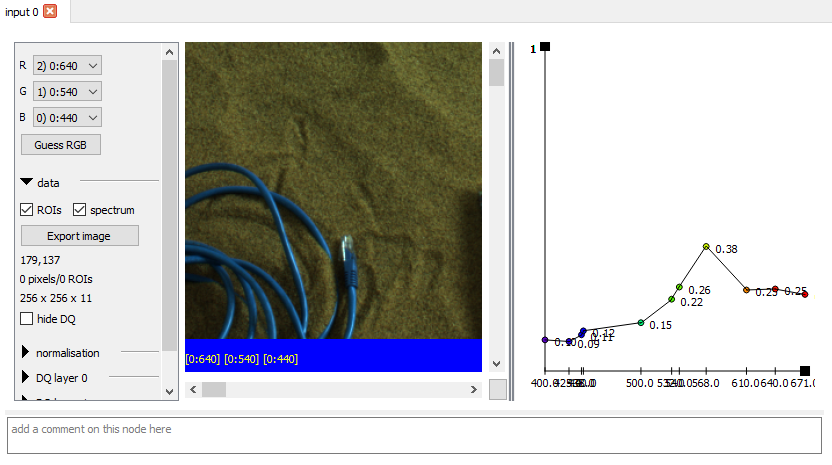
The screenshot isn't showing the cursor, unfortunately, but the spectrum is for the pixel under the cursor.
With PCOT version 0.12 (JOANEY HOW) and later, it's possible to show the spectrum for an area of pixels shown by a red square. This is done by selecting a value that isn't "1x1" in the Spectrum Region combo box. The spectrum plotted will show the mean and pooled standard deviation (by Rudmin's method, in which the pooled variance is the variance of the mean plus the mean of the individual pixel variances).
When a spectrum view is opened the image pane can be tiny - to fix this you can resize the PCOT window (or undocked node window), or drag the separator between the image and the spectrum (the two vertical bars). Each dot is shown with an approximation of its wavelength colour (using Dan Bruton's algorithm) or black if the wavelength is not visible.
- Export image saves the RGB-mapped image as a PDF, SVG or PNG. If a gradient has been plotted using the gradient node, it may add a legend to the image.
- Cursor coordinates are shown next, followed by number of pixels and ROIs in the image and the image dimensions (width x height x bands).
- The hide DQ disables the data quality overlays and hides their sections - data quality can be slow to draw.
Normalisation section
Nominally, the canvas channels are 0-1 with 0 being zero intensity and 1 being full intensity (so RGB 1,1,1 is white). Values outside the 0-1 range are clamped. However, this can be changed.
- The norm box selects the normalisation range:
- to all bands means that the normalisation range of each band for each pixel is the minimum and maximum of all the bands as a whole.
- to RGB means that the normalisation range is taken from the channels mapped to RGB in the canvas.
- independent means that each band is normalised independently, to its own range.
- none means no normalisation is done.
- If to cropped area is on, the range used for normalisation is taken from the portion of the image visible in the canvas.
Data quality layers
Each image has a set of data quality bits and an uncertainty value associated with each pixel of each band. Viewing this can be challenging. We make three "layers" of DQ data available: each works the same way:
- SRC specifies which band we are viewing the DQ or uncertainty for. If max is specified and we are viewing uncertainty, the maximum uncertainty across all bands is used. If sum, then the sum of the uncertainties is used. If a DQ bit is being shown, the intersection of those bits across all bands is used for both max and sum.
- DATA specifies what data is being shown:
- NONE specifies that the DQ layer is inactive.
- BIT:name options specify a particular DQ bit. These are subject to change, but are likely to include nodata, nounc (no uncertainty data), sat (saturated).
- UNC specifies that the uncertainty data should be shown.
- UNC>THRESH specifies that the layer should be full intensity for pixels where the uncertainty is above a threshold (see below).
- UNC<THRESH specifies that the layer should be full intensity for pixels where the uncertainty is below a threshold (see below).
- COL specifies the colour for the DQ layer.
- transp indicates the transparency of the layer
- contrast may help improve visibility (it is a simple power function)
- thresh is the threshold for the threshold DATA modes
- additive indicates that the data quality layers should be added to the RGB image rather than blended.
The right-click menu
There are several useful functions available in this menu, which pops up when you click the right mouse button.
Saving an image
Canvas images can be saved in several formats by selecting Save as image, PDF, SVG or PARC
Store/load view location
It is often useful to be able to view the same small area in different nodes. You can capture a canvas view's centre point and zoom and then load it in another node using the right-click context menu:
- Store canvas view location will store the centre point and zoom
- Load canvas view location when run in another canvas will load it, so you have the same view as the canvas in which you stored.
The loaded view may be slightly different because different nodes often have different canvas sizes.